Praxis 5162 Key Concepts to Know
Praxis Algebra I Category I: Principles of Algebra
This content category has about 23 questions. These questions account for 38% of the entire exam.
Let’s explore some specific concepts from this content category that are likely to appear on the test.
Parts of an Expression
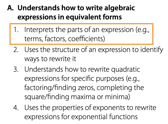
An expression is made up of one or more terms. A term is a single number or variable, or can be the product of numbers and variables.
Example: How many terms are in the expression 3xy + 4x -7?
This expression has three terms that are separated by addition and subtraction. They are 3xy, 4x, and -7.
A coefficient is the number that is multiplied by a variable in a term. For example, in the term 4x, the coefficient is 4. In the term -7xy, the coefficient is -7.
Expressions can be factored using a variety of strategies.
When factoring a polynomial, always look for the greatest common factor (GCF) first.
For example, the GCF of 3x³ – 6x² + 12x is 3x. Factor out the 3x so that the polynomial becomes 3x(x² – 2x + 4).
Binomials can often be factored using the difference of two squares if in the form a² – b² = (a – b)(a + b). For example, x² – 16 = (x – 4)(x + 4).
Trinomials of the form ax² + bx + c with a leading coefficient in which a = 1 can be factored by looking for two factors of c that add to equal b. For example, to factor x² + 5x + 6, think of two factors of 6 that add to equal 5. The two factors are 2 and 3, so this trinomial is factored into (x + 2)(x + 3).
For trinomials of the form ax² + bx + c with a leading coefficient in which a does not equal 1, use the “slide and divide” method.
For example, for 3x² – 7x – 6, there is not a GCF and a does not equal 1. Here’s how the “slide and divide” method would work with this equation:
- Slide the “a = 3” to multiply by the “c = -6.”
- Now use the trinomial x² – 7x – 18 and factor into (x – 9)(x + 2).
- Divide the -9 and 2 by the a = 3, so that the factors are now (x – 9/3)(x + ⅔).
- Simplify each. If the denominator remains, then “slide” the denominator “back up” to become the coefficient of x. The factors are now (x – 3)(3x + 2).
Add, Subtract, and Multiply Polynomials

A polynomial is an expression of one or more terms. It is possible to add, subtract, and multiply polynomials.
To add polynomials , combine like terms.
For example, to simplify (9x² – 4x + 5) + (-2x² + 6x – 2):
9x² + -2x² = 7x²
-4x + 6x = 2x
5 + -2 = 3
(9x² – 4x + 5) + (-2x² + 6x – 2) = 7x² + 2x + 3
To subtract polynomials, combine like terms, while being careful with negative signs.
For example, to subtract (5x² – 3x + 6) – (2x² – 5x + 1):
5x² – 2x² = 3x²
-3x – (-5x) = -3x + 5x = 2x
6 – 1 = 5
(5x² – 3x + 6) – (2x² – 5x + 1) = 3x² + 2x + 5
To multiply polynomials, multiply each term in one polynomial by each term in the other polynomial. This distribution method is commonly known as FOIL.
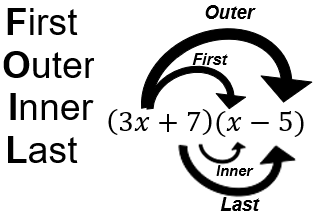
For example, to find the product of (3x-1)(2x+3):
- Multiply 3x(2x + 3) to get 6x² + 9x
- Multiply -1(2x + 3) to get -2x – 3
- Combine all terms so that (3x – 1)(2x + 3) = 6x² + 9x – 2x – 3 = 6x² + 7x – 3
Solve Linear Inequalities
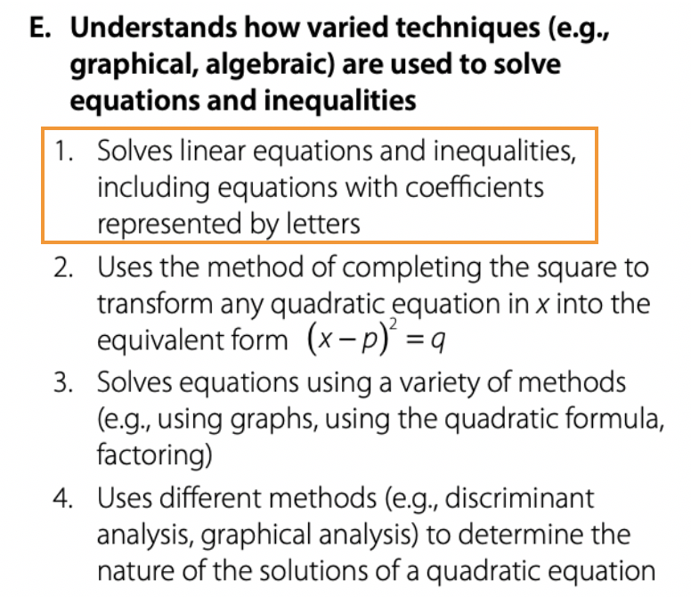
A linear inequality uses a linear function with one of the inequality symbols
(<, >, ≥, ≤) used to show which numbers would be solutions to the inequality.
Example 1: 2x – 3 > 1
- Use inverse operations to isolate the variable.
- Add 3 to each side: 2x – 3 + 3 > 1 + 3, 2 x > 4 .
- Divide each side by 2: the solution is x > 4.
- Any value of x that is greater than 4 would be a solution to the inequality.
Example 2: -3x – 4 ≤ 2x + 6
- Use inverse operations to isolate the variable.
- Add 4 to both sides, -3x – 4 + 4 ≤ 2x + 6 + 4 simplified becomes -3x ≤ 2x + 10.
- Subtract 2x from each side: -3x – 2x ≤ 10 becomes -5x ≤ 10.
- To isolate the variable, divide each side by -5. (Note: when multiplying or dividing an inequality by a negative value, the direction of the inequality sign will switch. For example, (-5x / -5) ≤ (10 / -5) becomes x ≥ -2.)
- Any value of x that is greater than OR equal to -2 is a solution to this inequality.
Completing the Square

One strategy for solving quadratic equations is to use completing the square to rewrite a quadratic equation. This is an alternative to solving quadratics by factoring or the quadratic formula.
Recall that a quadratic equation is in the form y = ax² + bx + c .
Example 1: Use completing the square to write x² – 6x + 7 = 2 as an equation of the form (x-p)² = q . (In this first example, notice how the leading coefficient is a = 1.)
First, bring all constants to the right side of the equation, and leave a space on the left side.
x² – 6x +__ = 2 – 7
x² – 6x +__ = -5
Next, take the b coefficient of the x term and divide it by 2 then square the result.
(b/2)² = (6/2)² = 3² = 9
Add this to each side of the equation.
x² – 6x + 9 = -5 + 9
The left side of the equation is now a perfect square trinomial. Factor the trinomial and simplify the left side of the equation.
(x – 3)² = 4
Example 2: Use completing the square to write 3x² – 4x – 6 = -1 as an equation of the form (x-p)² = q. (In this second example, notice that a does not equal 1.)
First, bring the constants to the right side of the equation, leaving a space on the left side.
3x² – 4x + __ = 5
Next, since a does not equal 1, divide all terms on both sides of the equation by a = 3.
(3x²) / 3 – (4x) / 3 + ___ = 5 / 3.
Simplify.
x² – (4x) / 3+ ___ = 5 / 3.
Next, take the b coefficient of the x term, divide it by 2, then square the result. (Recall that dividing a fraction by 2 is the same as multiplying by ½.)
(b/2)² = (-4/3 x ½)² = (-4/6)² = (-⅔)² = 4/9.
Add this to each side of the equation.
x² – (4x) / 3+ 4/9 = 5/3 + 4/9
The left side of the equation is now a perfect square trinomial and can be
factored. The right side can be simplified.
(x – 4/3)² = (15/9) + (4/9)
(x – 4/3)² = 19/9
Solve a System Consisting of a Linear Equation and a Quadratic Equation
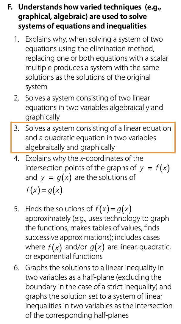
A system of equations consisting of one linear equation and one quadratic equation can be solved graphically or algebraically.
To solve the system graphically,
first graph each equation. The point(s) where the two equations intersect are the solutions to the system.
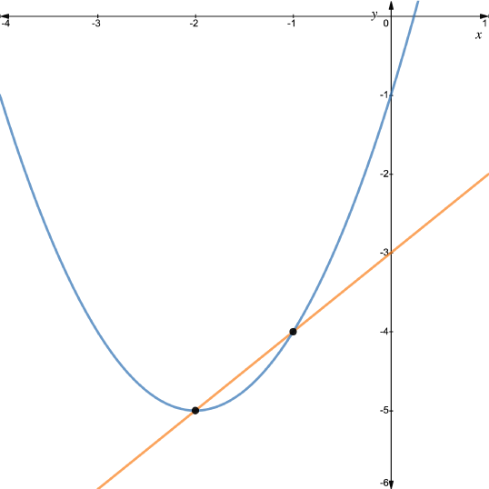
In the graph above, the two curves intersect at (-2, -5) and (-1, -4).
To solve the system algebraically,
follow these steps:
- Solve each equation for y.
- Set the equations equal to each other.
- Combine like terms to one side of the equation so that the equation then equals 0.
- Factor or use the quadratic formula to solve for x.
- Substitute the x-value(s) into one of the original equations to find the corresponding y-coordinate(s) for the point(s).
- Always check your solution(s) in one of the original equations.
Example: Solve the system below.
x – y = 3
y = x² + 4x – 1
First, solve each equation for y. So the linear equation becomes y = x – 3.
Next, set the equations equal so that x – 3 = x² + 4x – 1.
Combine like terms to one side so that one side of the equation equals 0.
0 = x² + 3x + 2.
Then, factor 0 = (x + 2)(x + 1)
Solve each factor for x, x + 2 = 0 becomes x = -2 and x + 1 = 0 becomes x = -1.
Substitute each x value into one of the original equations.
Using y = x² + 4x – 1
When substituting x = -2, y = (-2)² + 4(-2) – 1 = -5.
When substituting x = -1, y = (-1)² + 4(-1) – 1 = -4.
The solutions are (-2, -5) and (-1, -4).
Checking into x – y = 3, -2 – (-5) = 3 and -1 – (-4) = 3, so both solutions are valid.
Average Rate of Change of a Function
Average rate of change of functions is the slope of the function over a given value. For a nonlinear function, however, the average rate of change is not constant.

The slope formula is still used to find the slope of the line that connects between two points on the curve. A positive slope shows a positive rate of change while a negative slope shows a negative rate of change.
From a graph:
For the graph of f(x) = x³ – 2x², find the average rate of change from x = 2 to x = 3.
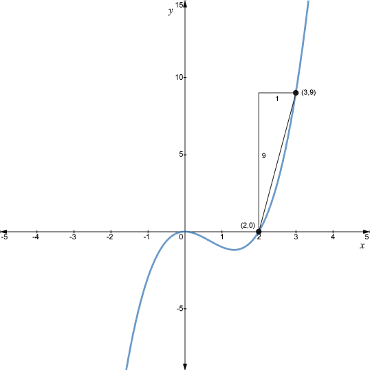
Look at the line segment that connects (2, 0) and (3, 9). To go from (2,0) to (3,9) you must rise 9 units and run to the right 1 unit, so the average rate of change is 9/1 or 9.
From a table:
Find the average rate of change from x = 0 to x = 3.

Using the slope formula [f(b) – f(a)] / [b – a], find the slope between (0, 5) and (3, 14).
The average rate of change over this interval is (14 – 5) / (3 – 0) = 9/3 = 3.
From a function:
Find the average rate of change of f(x) = x^(½) from x = 0 to x = 4.
Substitute into the function to find the values of f(0) and f(4).
f(0) = 0^(½) = 0 and f(4) = (4)^(½) = 2.
Using the points (0, 0) and (4, 2), the average rate of change is (2-0) / (4-0) = 2/4 = ½.
Calculating Intercepts and Slope of a Line
The x-intercept of a line is where the line crosses the x-axis. This can be found by setting the y value equal to zero, then solving for x.
The y-intercept of a line is where the line crosses the y-axis. This can be found by setting the x-value equal to zero, then solving for y.
The slope or steepness of a line is found using the formula:

Graph example:
The graph below represents the distance of a hot air balloon from the ground.
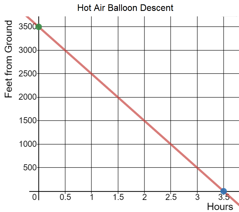
First, notice the units for x and y; the x-values represent hours, and the y-values represent the distance in feet of the hot air balloon from the ground. When interpreting any ordered pair that falls on the line, the values will represent (hours, feet).
The y-intercept is at (0 hours, 3500 feet), meaning the hot air balloon starts at 3,500 feet off the ground. The x-intercept is at (3.5 hours, 0 feet), meaning that it takes 3.5 hours for the hot air balloon to reach the ground.
The slope of the line measures the rate of change as feet/hour and will tell you how many feet per hour the hot air balloon descends. The slope of the line is negative, which tells you that the height of the hot air balloon is decreasing. The exact slope is -500 / 0.5, which means that the hot air balloon is getting closer to the ground at a rate of 1000 feet per hour.
Algebraic example:
You can also work to find the intercepts and slope of a function algebraically.
For the function f(x) = x – 2, find the x- and y-intercepts and the slope from x = -1 to x = 4.
To find the y-intercept, let x = 0, f(0) = 0 – 2 = -2.
The y-intercept is at (0, -2).
To find the x-intercept, let f(x) = y = 0. For this function, 0 = x – 2, x = 2 so the x-intercept is (2, 0).
To find the slope of the line find the (change in y values) / (change in x values):
(2 – -3) / (4 – -1) = 5 / 5 = 1.
And that’s some basic information about the Principles of Algebra content category of the Praxis Algebra I exam.
Praxis Algebra I Category II: Functions
This content category has about 18 questions. These questions account for 30% of the entire exam.
Let’s explore some specific concepts from this content category that are likely to appear on the test.
Domain and Range
The domain of a function is all of the x values of the function. The range of a function is all of the y values of the function. Domain and range can be found from a function rule, a graph, a set of ordered pairs or from a table.
From a graph:
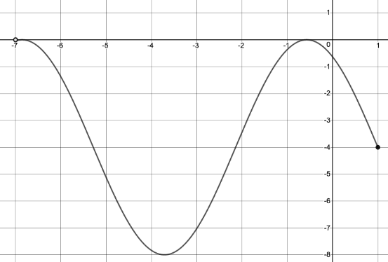
For the domain, the least x-value the graph touches is -7, but this point is included in the graph because of the open dot. The greatest x-value is 1. The domain is all x-values between -7 and 1, including 1 but not -7. This domain can be written as
D: -7 < x ≤ 1
For the range of the graph above, the least y-value is -8, and the greatest y-value is 0. The range is all y- values in between and including -8 and 0. This range can be written as R: -8 ≤ y ≤ 0.
From a function:
Find the domain and range of f(x) = x² – 3x + 2.
- Since this is a polynomial with no restrictions on the domain, the domain can be all real numbers.
- The range is also all real numbers.
Find the domain and range of f(x) = (x – 2) / (x + 3)
- This is a rational function, so at x = -3, the denominator equals 0, making the function undefined here due to a vertical asymptote on the graph. The domain of the function is all real numbers except x = -3.
- The range is all real numbers except y = 1, where a horizontal asymptote is located.
From a set of ordered pairs:
- Find the domain and range of the set {(2, 3), (-1, 2), (3, -4)}.
- The domain is the set of all x values: D = {-1, 2, 3}
- The range is the set of all y values: R = {-4, 2, 3}
From a table:

- The domain is the set of x values D = {-2, 3, 7}.
- The range is the set of y values R = {1, 3, 4}.
Odd and Even Functions
An even function is a function that when graphed has y-axis symmetry.
Algebraically, to identify if a function is even, substitute a (-x) in place of each (x) in the function. If the function is even, then f(-x) = f(x)
Example: Determine if f(x) = x² + 4 is even.
- Substitute (-x) in for each (x): f(-x) = (-x)² + 4 = x² + 4 = f(x).
- Since the original function results after substituting in the (-x), the function is even.
An odd function is a function that when graphed has symmetry about the origin. Algebraically, to identify a function as odd, substitute a (-x) in place of each (x) in the function. If the function is odd, then f(-x) = -f(x).
Example: Determine if the function f(x) = x³ – x is odd.
- Substitute (-x) in for each (x): f(-x) = (-x)³ – (-x) = -x³ + x.
- Factor out a negative one: f(-x) = -(x³ – x) = -f(x).
- Since the resulting function is -f(x) or negative of the original function, the function is odd.
It is possible for a function to be neither even or odd.
Example: Is f(x) = x³ – 1 even, odd, or neither?
First, substitute (-x) in for each (x). f(-x) = (-x)³ – 1 = -x³ -1. This is not the original function, so the function is not even.
To check if the function is odd, try to factor out a negative one: f(-x) = -(x³ +1). This is not the original function multiplied by negative one, so the function is not odd. This is an example of a function that is neither even or odd.
Write a Function
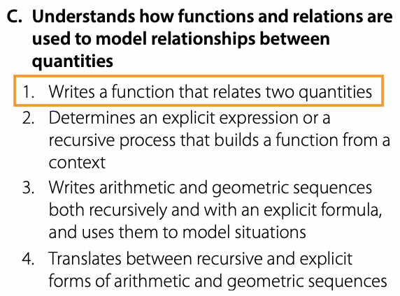
A function is a rule to represent a relationship between two quantities. A function can be written from a table of values.
Example 1: Given the table below, find the function rule that shows the relationship between x and f(x).

Notice that the y-intercept is at (0,3). As each x increases by two, each y-value increases by 4. This shows that the slope is m = 4/2 = 2.
The table represents a linear function which can be written in slope-intercept form, y = mx+b where m is the slope and b is the y-intercept.
The function that represents the relationship of the quantities in this table is
f(x) = 2x + 3.
Example 2: Using the table of values below, write a function to describe the relationship between x and f(x).

For this table, notice that each y value is multiplied by 2 as the x value increases by one. This is an example of an exponential function.
The y-intercept is located at (0, 4). The model for an exponential function is y = a(b)ˣ where a is the initial value and b is the change factor.
For this function, a = 4 and b = 2, so the function that represents this table’s relationship is f(x) = 4(2)ˣ.
Finding the Inverse
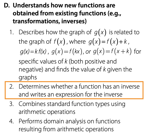
A function has an inverse if its graph passes the horizontal line test, meaning that a horizontal line can be drawn anywhere through the graph and only touch once.
Algebraically, for every y value, there is only one x value.
To find the inverse of a function:
- Let f(x) = y.
- Switch the x and y.
- Solve for the “new y.”
- Call y = f⁻¹(x).
Example: Find the inverse of f(x) = 2x – 5.
- First call f(x) = y, y = 2x – 5.
- Now, switch the x and y, so that x = 2y – 5.
- Solve for the “new y,” y = (x + 5) / 2.
- Call this new equation f⁻¹(x) = (x + 5) / 2.
Linear Functions vs. Exponential Functions
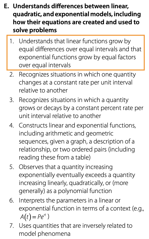
A linear function grows by a common difference, or the same number added or subtracted from the previous number.
For the linear function f(x) = 3x – 2, make a table of values.
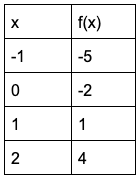
Notice how for every change in x of 1, the y-value, or output value, changes by 3.
An exponential function changes by equal factors or by multiplying by the same number.
For f(x) = 3ˣ, make a table of values.
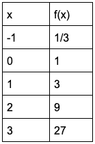
Notice how for every change in x of one, the change in the y-value, or the output, is multiplied by 3.
And that’s some basic information about the Functions content category of the Praxis Algebra I exam.
Praxis Algebra I Category III: Number and Quantity; Probability and Statistics
This content category has about 19 questions. These questions account for 32% of the entire exam.
Let’s explore some specific concepts from this content category that are likely to appear on the test.
Performing Operations with Exponents
There are many different properties for performing operations on exponents.
When adding or subtracting terms with exponents, only terms with like exponents may be added. For example, 3x² + 4x³ – x² = 2x² + 4x³.
When multiplying terms with exponents, the exponents can be added as long as the bases of the exponents are the same. For example, (4x³)(2x⁶) = 8x⁹.
When dividing terms with exponents, the exponents should be subtracted, as long as the bases of the exponents are the same. For example, (15x⁷) / (3x⁴) = 5x³.
When negative exponents result, it is important to make them positive by moving the term to the numerator or denominator, wherever it wasn’t located when negative. For example, 2/(x⁻³) becomes 2x³ when the x⁻³ is moved up to the numerator. In contrast, 4x⁻⁵ has the negative exponent in the numerator, so to make the exponent positive, move the term with the exponent to the denominator. This term becomes 4/(x⁵).
Rational exponents require the same rules. For example, x^(⅔) ∙ x^(⅘) requires that the exponents be added together.
In order to add ⅔ + ⅘ , first find a common denominator of 15 and rewrite each number. The sum becomes 10/15 + 12/15 = 22/15, so x^(⅔) ∙ x^(⅘) = x^(22/15).
Scatterplots
Scatterplots are used to graph data points that show how two quantitative
variables are related. The scatterplot can show how strong the relationship
between two variables are. In general, the x-axis has the independent variable while the y-axis has the dependent variable. The way the variables relate is called correlation.
There are three types of correlation: positive, negative, and no correlation.
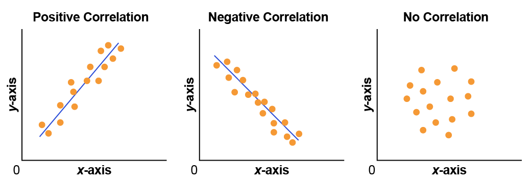
Positive correlation occurs when the dependent variables increase as the independent variables increase. An example of positive correlation would be a correlation between more hours studying and higher test grades. Points in the scatterplot will trend toward a positive slope.
Negative correlation occurs when one variable increases while the other variable decreases. One example of negative correlation would be a correlation between more exercise and a decrease in weight. Points in the scatterplot will trend towards a negative slope.
No correlation occurs when there is no observable trend or relationship between two variables and their points on their scatterplot. One example of two variables with no correlation or relationship would be height in inches and test scores.
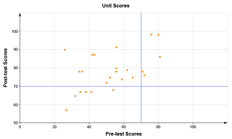
In the scatterplot below, the relationship between a student’s pre-test scores and post-test scores is graphed. Notice that as the pre-test scores increase, the post-test scores increase. This is an example of a scatterplot with positive correlation.
Correlation and Causation
Correlation is the direct connection or relationship between two things or quantities. Causation occurs when one event is caused or affected by another.
One example of positive correlation that is also causation would be that the longer you exercise, the more calories you burn. This is measurable, since the number of calories can be counted. As the minutes of exercise increase, so do the number of calories burned.
It is important to recognize that correlation does not necessarily mean causation .
Determining Probability

Probability is the likelihood of an event happening. The probability must be between 0 and 1. The closer the probability is to 1, the greater the likelihood of the event happening.
The probability of a simple event is finding the probability that a single event occurs. A simple event is one in which all outcomes are equally likely. For the purposes of predicting the probability of a given outcome, flipping a two-sided coin, throwing a six-sided die, and spinning a spinner with equal sections are all examples of simple events.
The probability is found by dividing the number of favorable outcomes by the number of possible outcomes. This needs to be simplified.
Example: Joe has 2 green, 4 blue, and 3 red marbles in a bag. What is the probability that he will grab a blue marble on his first reach into the bag?
- First, count the total number of possible outcomes. There are 2 + 4 + 3 = 9 marbles.
- Next, find how many favorable outcomes there are. In this problem, there are 4 possible blue marbles. The probability of grabbing a blue marble would be 4/9.
The probability of compound events is the probability that multiple events occur at the same time. The same formula is used as the one for finding the probability of simple events, but to find the probability of compound events, you multiply the probability of each independent event together.
Example: Madilyn and Kai are playing a board game in which they each roll two dice on their turn. What is the probability that Kai rolls two 5s?
- Calculate each event on its own. The probability of rolling a 5 on one die is ⅙. The probability of rolling a 5 on the second die is ⅙.
- To find the compound probability, multiply the probability of the two events together: (⅙)(⅙) = (1/36).
And that’s some basic information about the Number and Quantity; Probability and Statistics content category of the Praxis Algebra I exam.
